Example 1 Model green roofs internally and externally using SWMM
In this example, the hydrological performance of green roofs in a simple urban catchment is examined. The green roofs are first modeled externally using the SWMM’s green roof module, and then the resulted hydrograph is coupled with the SWMM catchment model using the functions provided by the toolbox. The result is then compared to that obtained by modeling green roofs internally using SWMM. The results of two cases are expected to be the same, as the toolbox is designed to update the parameters to accommodate the external modeling of green roofs and the same green roof model is used in both cases. The simulations are driven by a 60 mm SCS type III 24-hr design storm.
1. Original catchment without green roofs
The parameter of the original subcatchment before installing green roofs is stored in raw_catchment.inp. The modeled catchment only has a 0.5-acre impervious catchment, which drains runoffs from the catchment to the out. The catchment can be plotted by executing the code chunk that uses functions provided by swmmr.
# Load toolbox functions
source("interface_functions.R")

inp <- read_inp("./example/example1/raw_catchment.inp")

# Functions provided in swmmr are used for visualization
sub_sf <- subcatchments_to_sf(inp)
lin_sf <- links_to_sf(inp)
jun_sf <- junctions_to_sf(inp)
rg_sf <- raingages_to_sf(inp)

lab_coord <- sub_sf %>%
  sf::st_centroid() %>%
  sf::st_coordinates() %>%
  tibble::as_tibble()

lab_rg_coord <- rg_sf %>%
  {sf::st_coordinates(.) + 500} %>% # add offset
  tibble::as_tibble()

sub_sf <- dplyr::bind_cols(sub_sf, lab_coord)
rg_sf <- dplyr::bind_cols(rg_sf, lab_rg_coord)

ggplot() +
  # first plot the subcatchment and color continuously by Area
  geom_sf(data = sub_sf, aes(fill = Perc_Imperv), color = "black", alpha = 0.8) +
  scale_fill_gradient(low = "lightgreen", high = "indianred4") +
  geom_sf(data = lin_sf, colour = "blue", size = 1) +
  geom_sf(data = jun_sf, colour = "grey20", size = 2) +
  geom_label(data = sub_sf, aes(X, Y, label = Name), size = 3) +
  labs(x = "x-axis",
       y = "y-axis",
       fill = "Imperviousness\n(%)") +
  scale_fill_gradient(limits = c(0,100), low = "#009E73", high = "#D16103") +
  theme_bw(base_size = 10)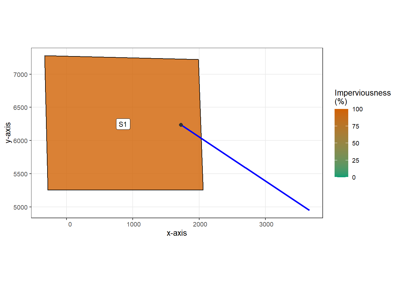
The run_swmm function provided by swmmr is used execute SWMM simulation. The outflow is store in test.txt in the current the current working directory and is stored in the raw_outflow variable using the read_outflow function as defined in the code chunk below.
run_swmm("./example/example1/raw_catchment.inp")

read_outflow <- function(fpath = "outflow.txt"){
  # Purpose: read simulated outflow hydrograph
  # Input:
  #    fpath = file path of the simulated outflow, which is defined in the [FILES] tab in SWMM input file
  # Output:
  #    a tibble stores the outflow hydrograph

  read_table(fpath, skip = 7) %>%
    transmute(datetime = ymd_hms(paste(Year, Mon, Day, Hr, Min, Sec)),
            flow = FLOW) %>%
    arrange(datetime)
}

raw_outflow <- read_outflow()
2. Green roofs modeled using SWMM’s green roof module
Assume the green roofs have a surface area of 0.25 acre (i.e., half of the catchment area). The SWMM model for the green roofs is SWMM_green_roof.inp. The outflow hydrograph from green roofs can be obtained using the run_swmm and read_outflow function.
run_swmm("./example/example1/SWMM_green_roof.inp")
SWMM_green_roof_outflow <- read_outflow()
The hydrograph is then saved in GR_outflow.txt using write_csv, and is later used as input flows to SWMM.
fname = "./example/example1/GR_outflow.txt"
write_csv(SWMM_green_roof_outflow, path = fname)
## Warning: The `path` argument of `write_csv()` is deprecated as of readr 1.4.0.
## Please use the `file` argument instead.
## This warning is displayed once every 8 hours.
## Call `lifecycle::last_warnings()` to see where this warning was generated.3. Catchment with green roofs modeled using SWMM’s green roof module
The catchment with green roofs is modeled using SWMM. The model is stored in SWMM_catchment_w_GR.inp. The simulation can be executed using the following code chunk. The simulated outflow is stored in the SWMM_catchment_w_GR_outflow variable
run_swmm("./example/example1/SWMM_catchment_w_GR.inp")
SWMM_catchment_w_GR_outflow <- read_outflow()
4. Incorporating externally-modeled green roof hydrograph into SWMM simulation
The information the toolbox needed for coupling GR_outflow.txt and raw_catchment.inp is stored in the file GI_plan.csv. It can be read using the read_GI_plan function in the toolbox.
GI_plan <- read_GI_plan("./example/example1/GI_plan.csv")

print(GI_plan)
## # A tibble: 1 x 6
## inflow_path outlet subcatchment_na~ per_area_rep imp_area_rep width_adj
## <chr> <chr> <chr> <dbl> <dbl> <dbl>
## 1 C:/Users/User/Documents/swmm_gi_toolbox/example/example1/GR_outflow~ 0 S1 0 0.25 115Six variables are defined.
- inflow_path: the path of the file that stores the outflow hydrograph from GI. The hydrograph will be used as input flows to SWMM.
- outlet: the node or the subcatchment that receives the inflow. 0 means the same outlet as the subcatchment is used.
- subcatchment_name: the name of the subcatchment, where GIs are installed.
- per_area_rep: pervious area represented by the inflow hydrograph, i.e., the pervious area modeled externally.
- imp_area_rep: impervious area represented by the inflow hydrograph, i.e., the impervious area modeled externally.
- width_adj: the subcatchment width parameter after modeled GIs externally. 0 means no change to subcatchment width.
The outflow hydrograph is input to SWMM using routing interface files. The interface file can be created using the write_routing_interface_file function provided by the toolbox.
# read the SWMM input file of the original catchment using swmmr::read_inp
inp <- read_inp("./example/example1/raw_catchment.inp")

# write routing interface file
routing_interface_path <- "./example/example1/routing_interface.txt"
write_routing_interface_file(GI_plan, inp, routing_interface_path)
## [1] TRUEwrite_routing_interface_file returns TRUE is the routing interface is created successfully. write_routing_interface_file takes three arguments.
- GI_plan: the tibble that stores the information needed for creating routing interface file; it is output of the
read_GI_planfunction. See explanations forread_GI_planabove. - inp: the object that corresponds to the input file read by
swmmr::read_inp. - routing_interface_path: the file path of the routing interface file to be created.
- flow_unit: The unit of the hydrograph. The default is “CFS” (cubic feet per second).
SWMM input file needs to be modified to accommodate the external modeling of green roofs. The modify_inp function provided by the toolbox can modify the inp object of the original catchment according to GI_plan.
new_inp <- modify_inp(GI_plan, inp, routing_interface_path)## `summarise()` ungrouping output (override with `.groups` argument)modify_inp returns the inp object corresponds to the catchment after GIs are modeled externally. It takes three arguments, which are the first three arguments of write_routing_interface_file. See the explanations above.
The modified SWMM input file can then created and executed using the write_inp and run_swmm functions provided by swmmr.
# write new input file
write_inp(new_inp, file = "./example/example1/test.inp")
# run simulation
run_swmm("./example/example1/test.inp")
# read outflow hydrograph
coupled_outflow <- read_outflow()
5. Compare the results of model green roofs externally and internally using SWMM
The two simulated outflow hydrographs, SWMM_catchment_w_GR_outflow and coupled_outflow, are expected to be the same. The following code chunk produces a figure that compares the hydrographs of the original catchment and the catchment with green roofs modeled internally and externally.
# create a tibble that stores the outflow hydrographs of three cases
# convert to long form for plotting
hydrographs <- tibble(
  datetime = raw_outflow$datetime,
  original = raw_outflow$flow,
  internal = SWMM_catchment_w_GR_outflow$flow,
  external = coupled_outflow$flow) %>%
  gather(case, value, -datetime) %>%
  mutate(case = factor(case, levels = c("original", "internal", "external"))) %>%
  filter(datetime <= ymd_hm("2020-06-02 00:00"))

# plot in the same figure, different cases are map to different colors and linetypes
ggplot(hydrographs, aes(datetime, value, linetype = case, color = case)) +
  geom_line(size = 0.65) +
  scale_color_manual(values = c("grey", "tomato3", "turquoise3")) +
  scale_linetype_manual(values = c("dashed", "solid", "dotdash"))+
  labs(x = "Time",
       y = "Flow rate [CFS]") +
  theme_classic(base_size = 12) +
  theme(legend.position = c(1,1),
        legend.justification = c(1,1),
        legend.key.width = unit(1.5, "cm"))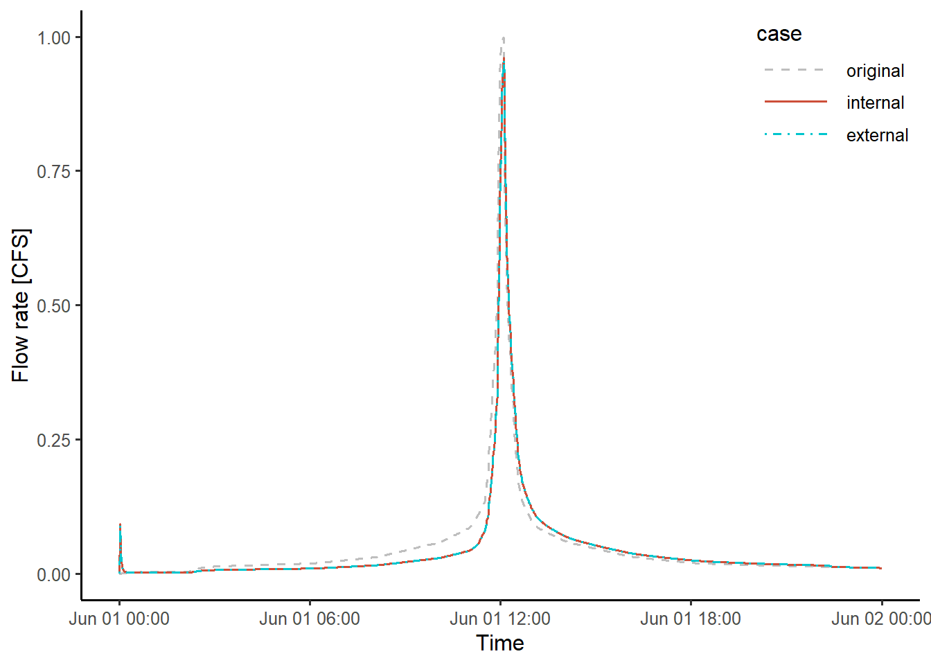
As expected, the hydrographs obtained for internal and external modeling cases are almost the same. This confirms the code worked as expected, i.e., the externally modeled outflow from green roofs is correctly written into the routing interface file, and the SWMM model parameters are correctly adjusted to represented the catchment areas without green roofs.
The difference in peak flow of the two modeling methods is -0.004 CFS, or -0.393%, and in runoff volume is -0.606 cubic feet, or -0.016%. The very small differences are mainly caused by rounding errors in computation and file processing.