Example 2 Installing multiple bioretention cells in different subcatchments
1. Overview
This example shows the procedure of using the toolbox when there are multiple subcatchments, and multiple green infrastructures (GIs) of different designs are installed in each subcatchment. The data used in this study can be found in example2 folder. The simulations are driven by a 60 mm SCS type III 24-hr design storm.
The studied catchment (in raw_catchment.inp) has three subcatchments. The surface area of them ranges between 0.5 acres to 0.9 acres, and the imperviousness ranges between 40% to 80%. The following code chunk generates a map of the catchment using functions provided by the swmmr package.
# Load toolbox functions
source("interface_functions.R")

inp <- read_inp("./example/example2/raw_catchment.inp")

# Functions provided by swmmr are used for visualization
sub_sf <- subcatchments_to_sf(inp)
lin_sf <- links_to_sf(inp)
jun_sf <- junctions_to_sf(inp)
rg_sf <- raingages_to_sf(inp)

lab_coord <- sub_sf %>%
  sf::st_centroid() %>%
  sf::st_coordinates() %>%
  tibble::as_tibble()

lab_rg_coord <- rg_sf %>%
  {sf::st_coordinates(.) + 500} %>% # add offset
  tibble::as_tibble()

sub_sf <- dplyr::bind_cols(sub_sf, lab_coord)
rg_sf <- dplyr::bind_cols(rg_sf, lab_rg_coord)

ggplot() +
  # first plot the subcatchment and color continuously by Area
  geom_sf(data = sub_sf, aes(fill = Perc_Imperv), color = "black", alpha = 0.8) +
  scale_fill_gradient(low = "lightgreen", high = "indianred4") +
  geom_sf(data = lin_sf, colour = "blue", size = 1) +
  geom_sf(data = jun_sf, colour = "grey20", size = 2) +
  geom_label(data = sub_sf, aes(X, Y, label = Name), size = 3) +
  labs(x = "x-axis",
       y = "y-axis",
       fill = "Imperviousness\n(%)") +
  scale_fill_gradient(limits = c(0,100), low = "#009E73", high = "#D16103") +
  theme_bw(base_size = 10)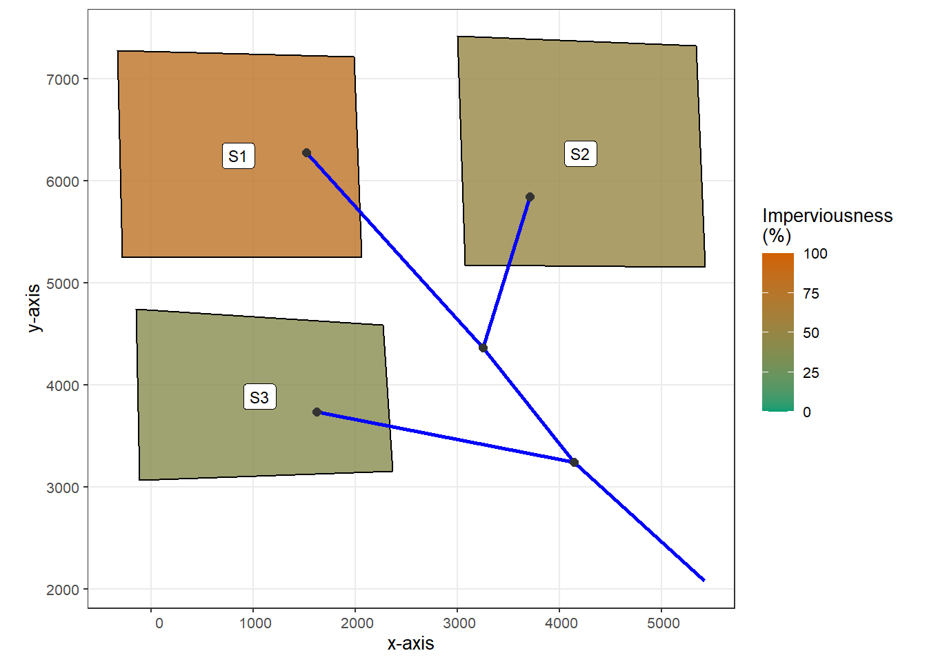
2. Outflow hydrographs from bioretention cells of different designs
Three different bioretention cell designs are considered in this study. The main difference is in the bioretention cell’s capture ratio. In each design, a bioretention cell is assumed to control 0.1 acres of the impervious area and its surface area is set to 3.4 %, 6.9 %, or 10.3 % of the controlled area. The outflow hydrographs from the bioretention cells are modeled using SWMM. The input files are named SWMM_bioretention1.inp, SWMM_bioretention2.inp, and SWMM_bioretention3.inp. The following code executes SWMM simulations, and write the simulated hydrographs into files named bc1_outflow.txt, etc.
read_outflow <- function(fpath = "outflow.txt"){
  # Purpose: read simulated outflow hydrograph
  # Input:
  #    fpath = file path of the simulated outflow, which is defined in the [FILES] tab in SWMM input file
  # Output:
  #    a tibble stores the outflow hydrograph

  read_table(fpath, skip = 7) %>%
    transmute(datetime = ymd_hms(paste(Year, Mon, Day, Hr, Min, Sec)),
            flow = FLOW) %>%
    arrange(datetime)
}

# Case 1: bioretention cells occupy 3.4 % of the catchment area
run_swmm("./example/example2/SWMM_bioretention1.inp")
bc1_outflow <- read_outflow()
fname = "./example/example2/bc1_outflow.txt"
write_csv(bc1_outflow, path = fname)

# Case 2: bioretention cells occupy 6.9 % of the catchment area
run_swmm("./example/example2/SWMM_bioretention2.inp")
bc2_outflow <- read_outflow()
fname = "./example/example2/bc2_outflow.txt"
write_csv(bc2_outflow, path = fname)

# Case 3: bioretention cells occupy 10.3 % of the catchment area
run_swmm("./example/example2/SWMM_bioretention3.inp")
bc3_outflow <- read_outflow()
fname = "./example/example2/bc3_outflow.txt"
write_csv(bc3_outflow, path = fname)
The following code chunk produces a figure that compares the outflow hydrograph generated for each bioretention design. The hydrographs varied considerably because of the modeling methods used for surface bypass flow and underdrain flow. More details on this issue can be found in this paper.
# Join the hydrographs into a single tibble
bc1_outflow$case = "BC design 1"
bc2_outflow$case = "BC design 2"
bc3_outflow$case = "BC design 3"

bc_outflow <- bc1_outflow %>%
  bind_rows(bc2_outflow) %>%
  bind_rows(bc3_outflow)

# Plotting
ggplot(bc_outflow, aes(datetime, flow, color = case, linetype = case)) +
  geom_line(size = 0.65) +
  scale_color_manual(values = c("grey", "tomato3", "turquoise3")) +
  scale_linetype_manual(values = c("dashed", "solid", "dotdash"))+
  labs(x = "Time",
       y = "Flow rate [CFS]") +
  theme_classic(base_size = 12) +
  theme(legend.position = c(1,1),
        legend.justification = c(1,1),
        legend.key.width = unit(1.5, "cm"))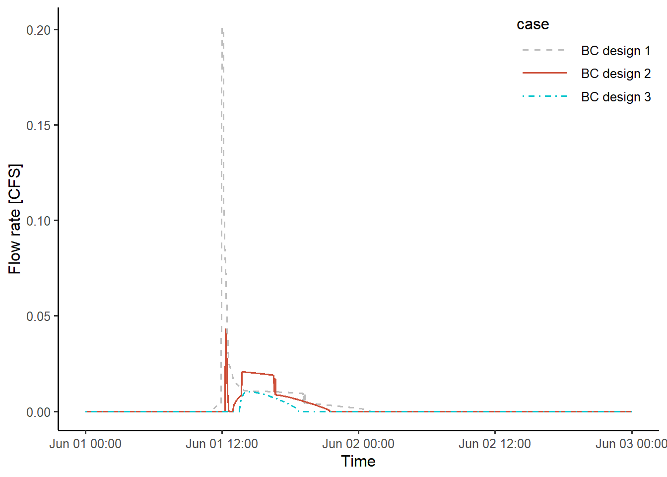
3. Creating bioretention cells implementation scenarios
In this study, three units of bioretention cells are planned for each subcatchment, and their designs are chosen randomly, i.e., different units of bioretention cells in the same subcatchment can have different designs.
The following code chunk creates a list of gi_plans to store the information needed for model coupling. The meaning of the column of the tibbles, such as inflow_path is explained in the Example 1. 50 different GI implementation scenarios are randomly generated, and in each scenario, three units of bioretention cells of different designs are randomly chosen for each subcatchment. Each bioretention cell controls an impervious area of 0.1 acres and drains to the same outlet as the subcatchment. The number of scenarios can be changed by setting the N value in the following code chunk.
set.seed(10)

inflow_paths <- paste0("./example/example2/bc", 1:3, "_outflow.txt")

N = 50 # Number of scenarios
gi_plans <- vector("list", 10) # list storing the random GI install plan
for (i in 1:N){
  gi_plans[[i]] <- tibble(
    inflow_path = sample(inflow_paths, 9, T),
    outlet = rep(0, 9),
    subcatchment_name = rep(c("S1", "S2", "S3"), each = 3),
    per_area_rep = rep(0, 9),
    imp_area_rep = rep(0.1, 9),
    width_adj = rep(0, 9)
  )
}
4. Creating routing interface files, modify SWMM input file, and run simulations
The function write_routing_interface_file provided by the toolbox can automatically create routing interface files to store the externally generated inflows that are readable by SWMM. The function modify_inp can modify the SWMM input files to account for the situation that runoffs from a part of the subcatchment are modeled externally. The functions provided by swmmr are used to run SWMM simulations.
The following code chunk derives outflow hydrograph at the catchment outlet for each bioretention implementation scenario. For each scenario, write_routing_interface_file function is first called to write SWMM interface file, modify_inp is then called to update the parameters of the catchment. Then write_inp and run_swmm are called to write SWMM input files and run simulations. The results are stored in the tibble outflows.
# Read the SWMM input file for the original subcatchment
inp <- read_inp("./example/example2/raw_catchment.inp")

# Create a list to store the simulated outflow hydrographs
outflows <- vector("list", N)
for (i in 1:N){

  # create a routing interface file
  gi_plan <- gi_plans[[i]]
  routing_interface_path <- "./example/example2/routing_interface.txt"
  write_routing_interface_file(
    GI_plan = gi_plan,
    inp = inp,
    routing_interface_path = routing_interface_path
  )

  # modify the object associated with SWMM input file
  new_inp <- modify_inp(
    GI_plan = gi_plan,
    inp = inp,
    routing_interface_path = routing_interface_path
  )

  # write the new SWMM input file
  new_inp_path <- "./example/example2/test.inp"
  write_inp(new_inp, file = new_inp_path)

  # run simulation
  run_swmm(new_inp_path)

  # get simulated outflow hydrograph
  outflows[[i]] <- read_outflow() %>%
    mutate(case = i)
}

# join the simulated hydrograph into a single tibble
outflows <- outflows %>%
  bind_rows()
5. Evaluate simulation results
The following figure shows the simulated hydrographs for all the scenarios using grey lines. The mean flow rate is shown using the blue line. Considerable variations can be observed among different bioretention implementation scenarios.
# Keep data for relatively high flow periods
data_plot <- outflows %>%
  filter(datetime <= ymd_hm("2020-06-02 00:00"))

# Get the mean hydrograph of all the scenarios
data_plot2 <- outflows %>%
  filter(datetime <= ymd_hm("2020-06-02 00:00")) %>%
  group_by(datetime) %>%
  mutate(mean_flow = mean(flow)) %>%
  ungroup()

# Plotting
ggplot() +
  geom_line(data = data_plot, aes(datetime, flow, group = case), color = "grey50", size = 0.5) +
  geom_line(data = data_plot2, aes(datetime, mean_flow), color = "blue", size = 0.8) +
  labs(x = "Time",
       y = "Flow rate [CFS]") +
  theme_bw()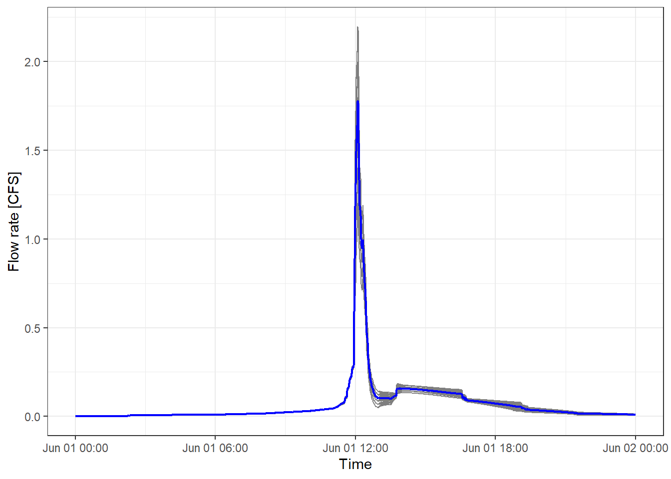
This example presents a workflow that multiple GIs are installed in different subcatchment. The two functions write_routing_interface_file and write_routing_interface_file keep track of each outflow hydrograph from GIs and aggregate the outflows drained to the same node of the drainage network before writing them into routing interface files.
The user needs to provide to the following information to the two functions, (1) a list of paths correspond to the hydrographs, (2) the destinations of the hydrographs, and (3) the name of the subcatchment, where the GIs locate, and (4) the associated changes to the catchment parameter after modeling GIs externally (e.g., changes to the pervious area of the subcatchment, changes to the width of the subcatchment, etc.) An example of the required information is provided in exmaple_gi_plan.csv. This file can be created using Microsoft Excel and similar spreadsheet software. This file can be read by the read_GI_plan function provided by the toolbox. Further details can be found in “Example 1” and the paper listed in the “About” section of this documentation.
write_csv(gi_plans[[1]], path = "./example/example2/exmaple_gi_plan.csv")